Pegasus Tutorial

Author: Yiming Yang, Rimte Rocher
Date: 2022-03-09
Notebook Source: pegasus_analysis.ipynb

Count Matrix File

For this tutorial, we provide a count matrix dataset on Human Bone Marrow with 8 donors stored in zarr format (with file extension ".zarr.zip").

You can download the data at https://storage.googleapis.com/terra-featured-workspaces/Cumulus/MantonBM_nonmix_subset.zarr.zip.

This file is achieved by aggregating gene-count matrices of the 8 10X channels using PegasusIO, and further filtering out cells with fewer than $100$ genes expressed. Please see here for how to do it interactively.

Now load the file using pegasus read_input function:

The count matrix is managed as a UnimodalData object defined in PegasusIO module, and users can manipulate the data from top level via MultimodalData structure, which can contain multiple UnimodalData objects as members.

For this example, as show above, data is a MultimodalData object, with only one UnimodalData member of key "GRCh38-rna", which is its default UnimodalData. Any operation on data will be applied to this default UnimodalData object.

UnimodalData has the following structure:

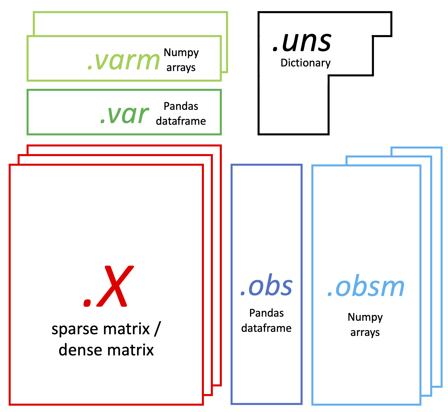
It has 6 major parts:

This dataset contains $48,219$ barcodes and $36,601$ genes.

Preprocessing

Filtration

The first step in preprocessing is to perform the quality control analysis, and remove cells and genes of low quality.

We can generate QC metrics using the following method with default settings:

The metrics considered are:

For details on customizing your own thresholds, see documentation.

Numeric summaries on filtration on cell barcodes and genes can be achieved by get_filter_stats method:

The results is a Pandas data frame on samples.

You can also check the QC stats via plots. Below is on number of genes:

Then on number of UMIs:

On number of percentage of mitochondrial genes:

Now filter cells based on QC metrics set in qc_metrics:

You can see that $35,465$ cells ($73.55\%$) are kept.

Moreover, for genes, only those with no cell expression are removed. After that, we identify robust genes for downstream analysis:

The metric is the following:

Please see its documentation for details.

As a result, $25,653$ ($70.09\%$) genes are kept. Among them, $17,516$ are robust.

We can now view the cells of each sample after filtration:

Normalization and Logarithmic Transformation

After filtration, we need to first normalize the distribution of counts w.r.t. each cell to have the same sum (default is $10^5$, see documentation), and then transform into logarithmic space by $log(x + 1)$ to avoid number explosion:

For the downstream analysis, we may need to make a copy of the count matrix, in case of coming back to this step and redo the analysis:

Highly Variable Gene Selection

Highly Variable Genes (HVG) are more likely to convey information discriminating different cell types and states. Thus, rather than considering all genes, people usually focus on selected HVGs for downstream analyses.

By default, we select 2000 HVGs using the pegasus selection method. Alternative, you can also choose the traditional method that both Seurat and SCANPY use, by setting flavor='Seurat'. See documentation for details.

We can view HVGs by ranking them from top:

We can also view HVGs in a scatterplot:

In this plot, each point stands for one gene. Blue points are selected to be HVGs, which account for the majority of variation of the dataset.

Principal Component Analysis

To reduce the dimension of data, Principal Component Analysis (PCA) is widely used. Briefly speaking, PCA transforms the data from original dimensions into a new set of Principal Components (PC) of a much smaller size. In the transformed data, dimension is reduced, while PCs still cover a majority of the variation of data. Moreover, the new dimensions (i.e. PCs) are independent with each other.

pegasus uses the following method to perform PCA:

By default, pca uses:

See its documentation for customization.

To explain the meaning of PCs, let's look at the first PC (denoted as $PC_1$), which covers the most of variation:

This is an array of 2000 elements, each of which is a coefficient corresponding to one HVG.

With the HVGs as the following:

$PC_1$ is computed by

\begin{equation*} PC_1 = \text{coord_pc1}[0] \cdot \text{HES4} + \text{coord_pc1}[1] \cdot \text{ISG15} + \text{coord_pc1}[2] \cdot \text{TNFRSF18} + \cdots + \text{coord_pc1}[1997] \cdot \text{RPS4Y2} + \text{coord_pc1}[1998] \cdot \text{MT-CO1} + \text{coord_pc1}[1999] \cdot \text{MT-CO3} \end{equation*}

Therefore, all the 50 PCs are the linear combinations of the 2000 HVGs.

The calculated PCA count matrix is stored in the obsm field, which is the first embedding object we have

For each of the $35,465$ cells, its count is now w.r.t. 50 PCs, instead of 2000 HVGs.

Nearest Neighbors

All the downstream analysis, including clustering and visualization, needs to construct a k-Nearest-Neighbor (kNN) graph on cells. We can build such a graph using neighbors method:

It uses the default setting:

See its documentation for customization.

Below is the result:

Each row corresponds to one cell, listing its neighbors (not including itself) from nearest to farthest. data_trial.obsm['pca_knn_indices'] stores their indices, and data_trial.obsm['pca_knn_distances'] stores distances.

Clustering and Visualization

Now we are ready to cluster the data for cell type detection. pegasus provides 4 clustering algorithms to use:

See this documentation for details.

In this tutorial, we use the Louvain algorithm:

As a result, Louvain algorithm finds 19 clusters:

We can check each cluster's composition regarding donors via a composition plot:

However, we can see a clear batch effect in the plot: e.g. Cluster 11 and 14 have most cells from Donor 3.

We can see it more clearly in its FIt-SNE plot (a visualization algorithm which we will talk about later):

Batch Correction

Batch effect occurs when data samples are generated in different conditions, such as date, weather, lab setting, equipment, etc. Unless informed that all the samples were generated under the similar condition, people may suspect presumable batch effects if they see a visualization graph with samples kind-of isolated from each other.

For this dataset, we need the batch correction step to reduce such a batch effect, which is observed in the plot above.

In this tutorial, we use Harmony algorithm for batch correction. It requires redo HVG selection, calculate new PCA coordinates, and apply the correction:

The corrected PCA coordinates are stored in data.obsm:

pca_key is the representation key returned by run_harmony function, which is equivalent to string "pca_harmony". In the following sections, you can use either pca_key or "pca_harmony" to specify rep parameter in Pegasus functions whenever applicable.

Repeat Previous Steps on the Corrected Data

As the count matrix is changed by batch correction, we need to recalculate nearest neighbors and perform clustering. Don't forget to use the corrected PCA coordinates as the representation:

Let's check the composition plot now:

If everything goes properly, you should be able to see that no cluster has a dominant donor cells. Also notice that Louvain algorithm on the corrected data finds 16 clusters, instead of the original 19 ones.

Also, FIt-SNE plot is different:

You can see that the right-hand-side plot has a much better mixture of cells from different donors.

Visualization

tSNE Plot

In previous sections, we have seen data visualization using FIt-SNE. FIt-SNE is a fast implementation on tSNE algorithm, and Pegasus uses it for the tSNE embedding calculation. See details

UMAP Plot

Besides tSNE, pegasus also provides UMAP plotting methods:

Below is the UMAP plot of the data using umap method:

Differential Expression Analysis

With the clusters ready, we can now perform Differential Expression (DE) Analysis. DE analysis is to discover cluster-specific marker genes. For each cluster, it compares cells within the cluster with all the others, then finds genes significantly highly expressed (up-regulated) and lowly expressed (down-regulated) for the cluster.

Now use de_analysis method to run DE analysis. We use Louvain result here.

By default, DE analysis runs Mann-Whitney U (MWU) test.

Alternatively, you can also run the follow tests by setting their corresponding parameters to be True:

DE analysis result is stored with key "de_res" (by default) in varm field of data. See documentation for more details.

To load the result in a human-readable format, use markers method:

By default, markers:

See documentation for customizing these parameters.

Let's see the up-regulated genes for Cluster 1, and rank them in descending order with respect to log fold change:

Among them, TRAC worth notification. It is a critical marker for T cells.

We can also use Volcano plot to see the DE result. Below is such a plot w.r.t. Cluster 1 with MWU test results (by default):

The plot above uses the default thresholds: log fold change at $1$ (i.e. fold change at $2$), and q-value at $0.05$. Each point stands for a gene. Red ones are significant marker genes: those at right-hand side are up-regulated genes for Cluster 1, while those at left-hand side are down-regulated genes.

We can see that gene TRAC is the second to rightmost point, which is a significant up-regulated gene for Cluster 1.

To store a specific DE analysis result to file, you can write_results_to_excel methods in pegasus:

Cell Type Annotation

After done with DE analysis, we can use the test result to annotate the clusters.

infer_cell_types has 2 critical parameters to set:

infer_cluster_names by default uses threshold = 0.5 to filter out candidate cell types of scores lower than 0.5.

See documentation for details.

Below is the cell type annotation report for Cluster 1:

The report has a list of predicted cell types along with their scores and support genes for users to decide.

Next, substitute the inferred cluster names in data using annotate function:

So the cluster-specific cell type information is stored in data.obs['anno'].

The anno_dict can be either a list or a dictionary. If provided a list (which is the case here), Pegasus will match cell types with cluster labels in the same order. Alternatively, you can create an annotation dictionary with keys being cluster labels and cell types being values.

In practice, users may want to manually create this annotation structure by reading the report in celltype_dict. In this tutorial, we'll just use the output of infer_cluster_names function for demonstration.

Now plot the data with cell types:

Raw Count vs Log-norm Count

Now let's check the count matrix:

You can see that besides X, there is another matrix raw.X generated for this analysis. As the key name indicates, raw.X stores the raw count matrix, which is the one after loading from the original Zarr file; while X stores the log-normalized counts.

data currently binds to matrix X. To use the raw count instead, type:

Now data binds to raw counts.

We still need log-normalized counts for the following sections, so reset the default count matrix:

Cell Development Trajectory and Diffusion Map

Alternative, pegasus provides cell development trajectory plots using Force-directed Layout (FLE) algorithm:

Moreover, calculation of FLE plots is on Diffusion Map of the data, rather than directly on data points, in order to achieve a better efficiency. Thus, we need to first compute the diffusion map structure:

By default, diffmap method uses:

In this tutorial, we should use the corrected PCA matrix, which is specified in pca_key. The resulting diffusion map is in data.obsm with key "X_diffmap":

Now we are ready to calculate the pseudo-temporal trajectories of cell development. We use fle here:

And show FLE plot regarding cell type annotations:

Save Result to File

Use write_output function to save analysis result data to file:

It's stored in zarr format, because this is the default file format in Pegasus.

Alternatively, you can also save it in h5ad, mtx, or loom format. See its documentation for instructions.

Read More...